


![]() n the early 1980s, the research group at Hammersmith Hospital in London succeeded in imaging the brain with such an excellent spatial and contrast resolution that they could compare their images with slices seen before only in necropsy. They used inversion-recovery (IR) pulse sequences [Bydder 1982].
n the early 1980s, the research group at Hammersmith Hospital in London succeeded in imaging the brain with such an excellent spatial and contrast resolution that they could compare their images with slices seen before only in necropsy. They used inversion-recovery (IR) pulse sequences [Bydder 1982].
In IR sequences, the initial magnetization is turned around by a 180° pulse. Thus, the recovery starts with a negative value, reaches 0 after 0.69 times the respective T1, then becomes positive and returns to its equilibrium after approximately five times T1 (Figure 10-08 top).
At some stage during this period, a 90° pulse is transmitted, which changes the partly recovered longitudinal magnetization into observable transverse magnetization. Commonly this is followed by another 180° pulse which creates a spin echo.
A detailed description of this pulse sequence can be found in Chapter 4.
 In reality, the initial negative magnetization is lost due to the calculation of the magnitude or modulus image (solid lines in Figure 10-08 top) from the real and imaginary signals, which is the standard procedure on most systems. Therefore, negative signals are recorded as positive signals of the same strength, and the signal is positive on either side of the null point. Image contrast in IR sequences reflects this behavior (Figures 10-08 and 10-09).
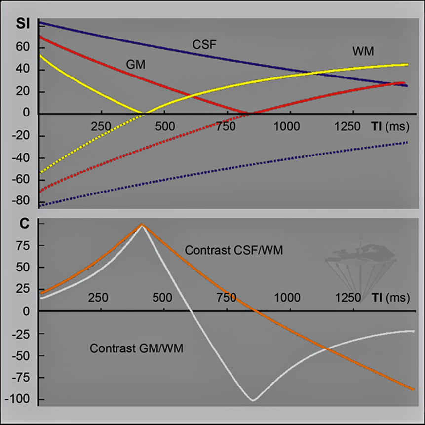
Figure 10-08:
Contrast is one of the major concerns in medical imaging.
Graph top: Relative sgnal-intensity (SI) behavior of an inversion-recovery sequence with a repetition time TR = 2000 ms, B₀ = 1.5 T. Note that until 0.69 × T1 has been reached, the signal is negative (dotted lines). The solid lines depict the IR signal intensity behavior in reality (magnitude image): the (positive) signal decreases to zero, then increases again until it reaches equilibrium.
Graph bottom: Contrast between gray and white matter and CSF in the same inversion-recovery experiment. There is poor contrast with short TI. It then increases and reaches a peak (in this case) at approximately 400 ms. Immediately afterwards, there is a sharp drop in gray/ white-matter contrast; it disappears completely, and then turns negative, reaching another peak. With long inversion times, it disappears again. CSF/white-matter contrast behaves similarly. Note that peaks of optimal contrast can be very close to zero contrast. When looking for pathology, this means that lesions may easily be overlooked if wrong inversion times are chosen.
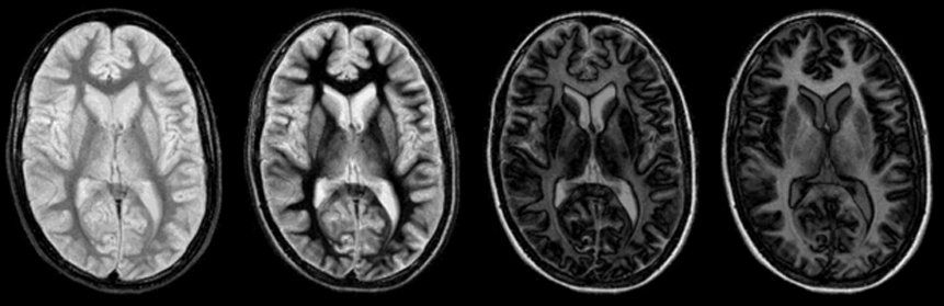
Figure 10-09:
The unexpected and abrupt contrast changes of an IR pulse sequence (cf. Figure 10-08): four images with increasing TI. One of the main problems (and advantages) of the IR sequence is that its contrast behavior can change dramatically with only minimal changes of the inversion time.

Figure 10-09-Video:
Animation: In all images, TR = 4000 ms (different from the graph in Figure 10-08). TI from 100 ms to 2000 ms, increasing in steps of 100 ms.
Simulation software: MR Image Expert®
To retain the signal information, a reference image is needed so that the phase in each pixel can be compared. An interlaced IR/PS sequence is one way of achieving this.
Images with long inversion times (TI) have hardly any contrast between neighboring tissues, except the one created by differences in proton density, whereas images with short TI show high contrast.
Like partial saturation sequences, IR emphasizes the longitudinal relaxation time T1. The intensity of an averaged signal can be calculated with the following equation:
where SI is signal intensity, K is a constant comprising bulk flow, diffusion, perfusion and other parameters, ρ is proton density, M₀ is magnetization at time 0, TI is the inversion time, TR is the repetition time, and T1 is the longitudinal relaxation time.
The signal intensity for a given T1 is strongly dependent on inversion and repetition times.
The IR sequences implemented in clinical machines add a second 180° pulse after the 90° pulse to rephase T2 influences. In this way, clinical IR images are also affected by T2. T2 is not meant to be a primary source of contrast in IR imaging; however, if a long TR and a long TE are chosen, IR images may mimic in part T2-weighted SE contrast.
If a shorter TR is chosen than the T1 of a particular component of the sample, it can happen that — at a certain TI, which is shorter than T1 — the relative signal intensity of this tissue component will be higher than that of a neighboring component with a shorter T1. This complicated and ambiguous contrast behavior is best understood from the curves and pictures in Figures 10-08 and 10-09.
The graphs and images show that the gaps between no contrast and high contrast are very small. If there are no unpredictable pathological changes present in the sample, contrast can be foretold.
Problems arise when unknown lesions are suspected. To avoid false interpretations of MR images, several pictures at different TI are desirable. This, however, prolongs imaging and examination times.
It is possible to produce several images with different TI values in a single interval using a special IR sequence, but the signal-to-noise ratio of this sequence is reduced because flip angles of ≤90° are applied for each excitation [⇒ Graumann 1987, ⇒ Young 1987].
Usually, IR images are acquired as multislice pictures. This means that several parallel slices, rather than one single slice, are imaged at a time. This is an elegant way to save time and shorten an examination, and greatly increases the efficiency of IR examinations, which are very time consuming.
The pulse sequence used for multislice IR is the BIR (balanced IR) sequence, which is also known as MDEFT (modified driven-equilibrium Fourier transformation). These sequences provide superior T1-weighted contrast to T1-weighted SE sequences.


|

|
|---|