


 he chemical-shift artifact is caused by the difference in resonance frequency experienced by protons in different chemical environments. Protons contained in fat and water environments are separated by 3.5 ppm. Both the frequency and slice encoding processes use frequency information. The signals from fat and water protons at the same position will result in different frequencies and therefore a relative shift of one of the signal components (Figure 11-02 and Figure 17-11).
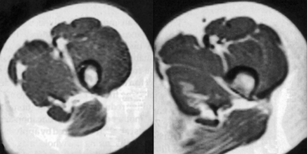
Figure 17-11:
High field strength (1.5 T) MR images with chemical shift artifacts in the readout direction, which is oriented vertically in the image. The chemical-shift artifact is visible as a black rim between fat and muscle.
Since this is a frequency-dependent artifact, the effect will be more pronounced at high and ultrahigh fields (1.5 T, 3.0 T, and more), with displacements of several pixels being visible in the readout direction. The artifact can be reduced by using stronger gradients, but this has the unfortunate side effect of decreasing the signal-to-noise ratio.
The problem can be overcome by suppressing one or other of the components prior to collecting each line of data. This can be done either by using presaturation techniques (which require good static field homogeneity) [⇒ Femlee 1987] or by using one of a number of add-subtract schemes (which increase the imaging time) [⇒ Dixon 1984, ⇒ Szumowski 1988].
In gradient-echo studies, changes in the echo time lead to changes in the relative phases of the fat and water components of the signal, as we have seen in Chapter 11. This can be used to change the contrast in the image or as the basis of a fat-suppression scheme [⇒ Williams 1989].
Sometimes well-defined black contours following anatomical structures are seen. These artifacts are another class of chemical-shift artifacts. Pulse sequences prone to such artifacts are inversion-recovery and gradient-echo sequences. The water and fat signals can be in-phase or out-of-phase (cf. fat-suppression technique in Chapter 11).
If this happens accidentally in volume elements with partial volume effects between water-rich and lipid-rich organs, the signal disappears and artifactual contours are seen (Figure 17-12). To avoid these contours, in-phase echo times must be used (cf. Figure 11-03).
Alternatively, the examination should be performed with SE sequences whose 180° pulses refocus the phase shifts.
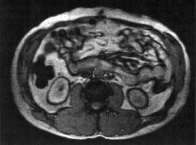
Figure 17-12:
Black boundary artifacts in the abdomen. Gradient-echo sequence with an echo time of 16 ms.
The truncation artifact is also known as ringing or Gibbs artifact.
It appears as parallel striations, close to interfaces between tissues with different signal intensities, such as fat-muscle or CSF-spinal cord. Because these lines mimic regular structures, they can present interpretation problems if they are not recognized as artifacts.
Truncation artifacts are particularly severe when small image matrices are used and can be reduced by simply using a larger image matrix.
Oversampling, while having no effect on the intensity of the truncation artifacts, does reduce their spacing which often results in the artifact becoming blurred and imperceptible.
Truncation artifacts are most commonly seen in the phase-encoding direction since increasing the matrix in this direction results in an undesirable increase in scan time. A combination of suitable scan orientation and increasing the data matrix in the frequency-encoding direction usually reduces the artifact to a tolerable level (Figure 17-13).
These artifacts can also be reduced by applying a low pass filter; but as with all filtering the whole image, and not just the artifact, will be affected.
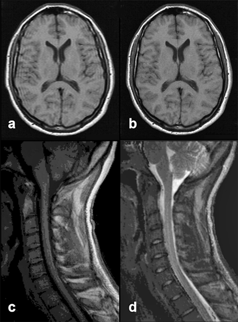
Figure 17-13:
Truncation artifacts.
Top: (a) 60% acquisition with artifacts. (b): 80% acquisition, no artifacts visible.
Bottom: Truncation artifact mimicking syringo-myelia. (c) T1-weighted, (d) T2-weighted image.
Aliasing artifacts are also known as backfolding, foldover, phase wrapping, or wrap around artifacts.
Aliasing causes data which lie outside the specified field-of-view to be wrapped back into the image. It can occur in both the phase and frequency encoding directions.
Aliasing can also be a k-space artifact (Figure 17-17).
 In the frequency-encoding direction the artifact results from the presence of signals with too high a frequency being mispositioned.
According to the Nyquist theorem, frequencies must be sampled at least twice per cycle in order to reproduce them accurately. Depending on the detection scheme used, the data can be folded back into the image on the same or on the opposite side.
These high-frequency signals can be removed with a filter, but the response of such a filter will not exactly match the desired frequency range (the image bandwidth), leading to some artifact still being present or to a loss of signal at the edges of the image.
This problem can be overcome by doubling the amount of data collected (oversampling), either by doubling the sampling rate to the critical sampling frequency (Nyquist frequency) or by doubling the acquisition time.
The latter scheme has the advantage of also improving the signal-to-noise ratio by √2. We can then apply a filter which will remove all frequencies outside of the new image bandwidth but which will have no effect on the frequencies that correspond to the desired field of view (Figure 17-14).
After the Fourier transformation the outer quadrants of the oversampled data are discarded, leaving us with the original field-of-view and no artifacts (Figure 17-14, bottom).
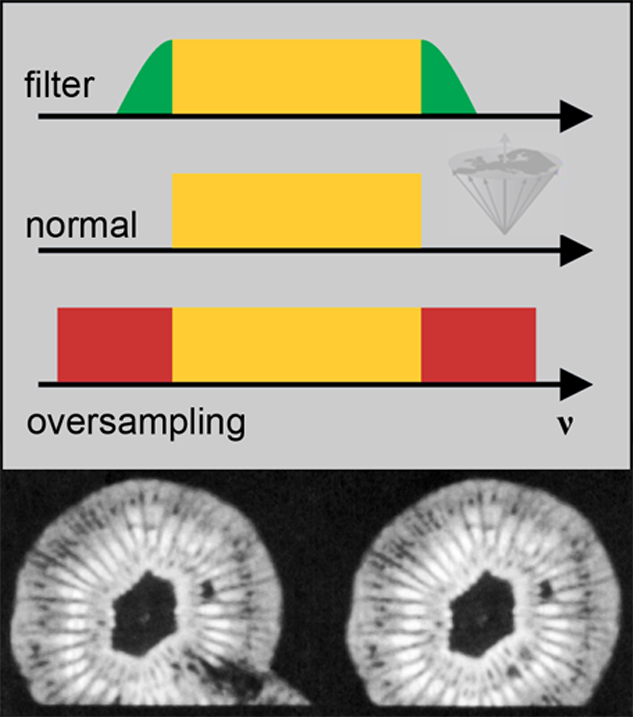
Figure 17-14:
Graph: Relation between the filter (top), the image frequencies for normal sampling (middle), and oversampling (bottom).
Bottom: Image of a kiwi fruit: (left) result of oversampling, and (right) normal sampling. In both cases, the frequency gradient was orientated vertically. In the left-hand image aliasing of signal originating from outside the specified field of view results in the artifact visible at the bottom.
ν = frequency.
In the phase-encoding direction aliasing results in signal from outside the field of view being folded back into the image on the opposite side, because the two positions will produce identical phases.
Oversampling can also be applied to the phase-encoding direction, but will double the imaging time (since twice as many phase-encoding steps are required); thus it is little used.
The usual practical solution is to orientate the phase encoding direction in the image in such a way that no anatomical structures extend beyond the image boundaries in this direction (Figure 17-15). If this is not possible, a surface coil can be used to limit the volume from which the signal is obtained. In 3D imaging, the backfolding can occur in both of the phase-encoded directions.
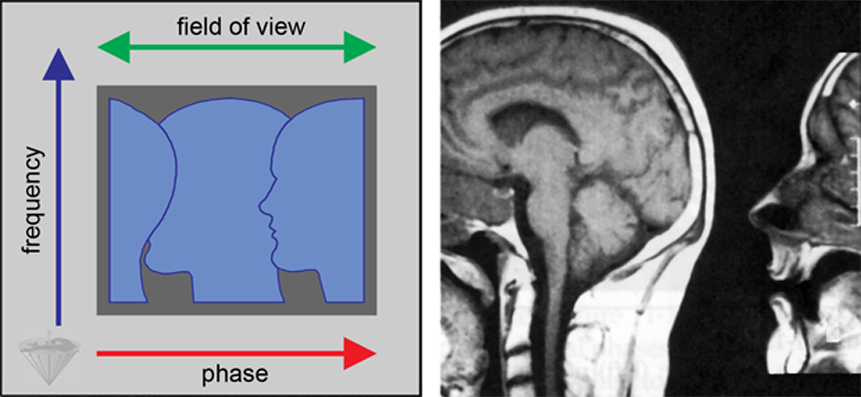
Figure 17-15:
Backfolding artifact resulting from the sample being larger than the field of view in the phase encoding direction, which is orientated left-right in this example.
The MR signal is detected using a receiver which has two channels, with the reference signal to the second channel being phase-shifted by exactly 90° with respect to the reference used for the first channel.
Any maladjustment of this phase-shift results in a ghost image, which is rotated about both the x- and y-axes with respect to the main image (Figure 17-16).
It can be eliminated by adjusting the phase and gain of the receiver, which is most easily done by trying to minimize the quadrature peak in a transformed, off-resonance signal.
Figure 17-16:
Quadrature artifact resulting from an incorrectly adjusted receiver.
The data in each individual pixel of the final MR image after Fourier transformation contains information from all points in k-space.
Thus any, even minor, disintegration of k-space such as bad data points or spikes can easily corrupt the entire final MR image and create image artifacts [⇒ Mezrich 1995].
Two of them are shown in Figure 17-17 and Figure 17-18.
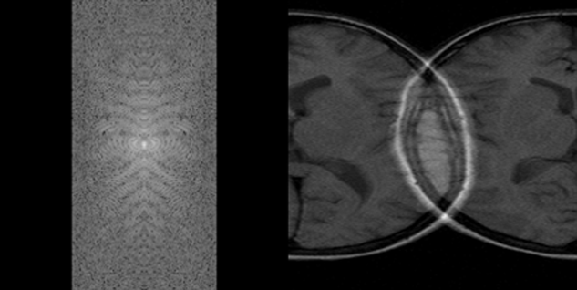
Figure 17-17:
k-Space artifacts: Aliasing or wrap-around artifact.
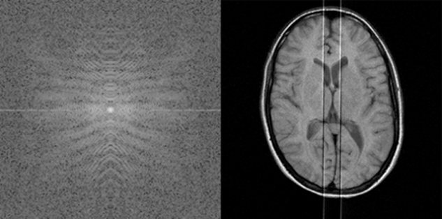
Figure 17-18:
k-Space artifacts: Radiofrequency feedthrough artifact.


|

|
|---|