02-08 The Magnetic Resonance Signal

To excite a spin system, one can expose the spins to a continuous elec­tro­mag­ne­tic wave of the right frequency. However, the method most commonly chosen for excitation of atomic nuclei in a magnetic field is to apply radiowaves of high in­ten­si­ty during a short period of time (pulsed magnetic resonance).

The frequency of these RF waves should be equal to, or close to, the Larmor fre­quen­cy of the nuclei. Viewed from the rotating coordinate system (Figure 02- 12 top), this re­sults in a rotation of the magnetization away from the direction of the external field (Fi­gu­re 02-12 center and bottom).

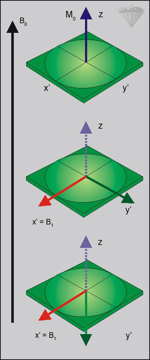
Figure 02-12: Top: At equilibrium there is one stationary mag­ne­tic moment, M0, directed along B0. Center: A 90° pulse. Bottom: A 180° pulse inverts the mag­ne­ti­za­tion. To understand this, we have to re­mem­ber that spins at the re­so­nan­ce fre­que­ncy are stationary in the rotating frame, implying a zero effective mag­ne­tic field. Therefore, the only field the spins experience is the B1 field, which is the field cre­a­ted by the RF pulse. The spins ro­ta­te about B1 in the same way as they rotate about B0 in the sta­ti­o­na­ry frame of reference. In other words, prior to the RF pul­se, the spins rotate about B0 which is aligned along the z-axis (Fi­gu­re 02-12 top). At this point, there is no net mag­ne­ti­za­tion in any direction within the x'-y' plane. The RF pulse then tips the net mag­ne­ti­za­tion away from the z-axis, to­wards the x'- and y'-axes of the ro­ta­ting frame.

Following the pulse, the spins are still precessing about B0, but their pre­ces­sion is no longer random; they precess in phase, and a net magnetization is pro­du­ced in the x'-y' plane. This magnetization is aligned along the y'-axis following a 90° pulse along x'. For a given RF intensity, the pulse angle is determined by the duration of the RF pulse. The duration of a 180° pulse is twice as long as that of a 90° pulse. Figure 02-12 (center) shows the situation for a 90° pulse, Figure 02-12 (bottom) for a 180° pulse that inverts the magnetization.

In the standard stationary frame of reference, we now have a component of mag­ne­ti­za­tion rotating at the Larmor frequency perpendicularly to B0 (= lon­gi­tu­di­nal mag­ne­ti­za­tion) in the x'-y' plane (= transverse magnetization). According to Faraday’s law of in­duc­tion, this transverse magnetization can induce a voltage in the receiver coil sur­roun­ding our sample.

When the excitation pulse is switched off, the spins start returning to their equi­li­bri­um and emit a signal. The signal that is received from a homogeneous sample in a ho­mo­ge­ne­ous magnetic field typically appears as shown in Figure 02-13a. It is called free induction decay, or FID, of the system. It looks like a damped oscillation.

If the magnetic field is not homogeneous, dif­fe­rent parts of the sample ex­pe­ri­en­ce different field strengths, and thus different parts of the sample will show dif­fe­rent Lar­mor frequencies, leading to a more complicated FID (Figure 02- 13b).

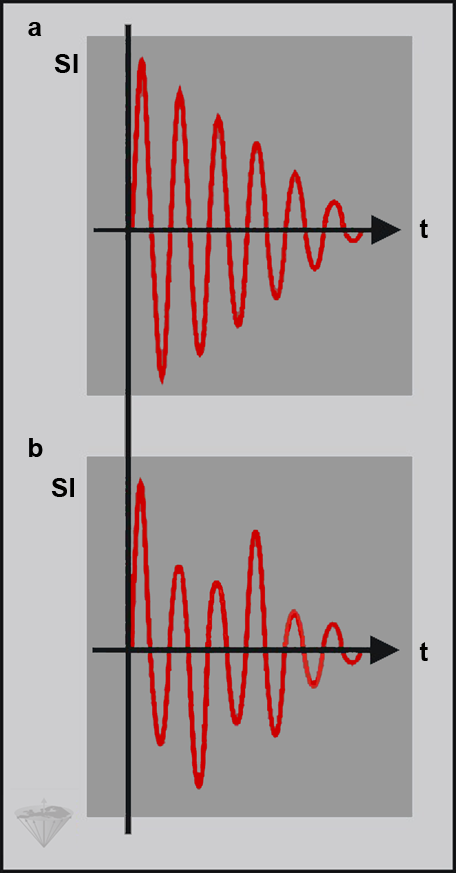
Figure 02-13:
The free induction decay (FID) (a) of a sample of pure water, (b) of a sample of water containing additional components. Usually, FIDs are far more complex than shown in these examples (SI = signal intensity; t = time).