• Chapter 7 • Contents
  Introduction The Optical Equivalent MR Imaging and k-Space Filling k-Space and Image Reconstruction 

---

07-03 MR Imaging and k-Space

hat we have said about optical lenses holds, in a similar way, for k-space in MR imaging (Figure 07-05).

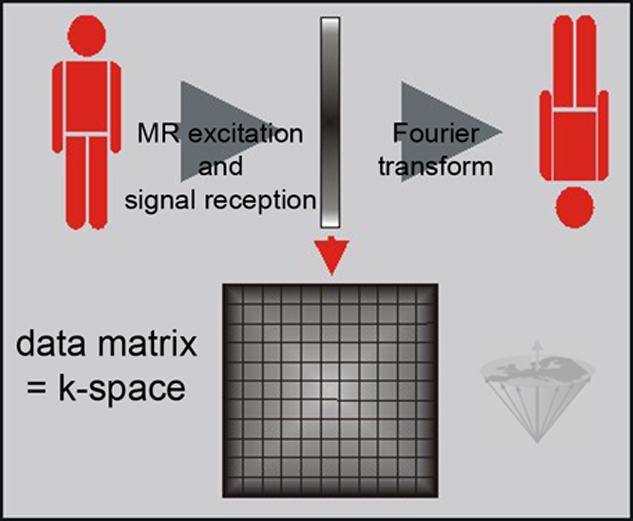
Figure 07-05:
From lens to MR imaging. If you compare this figure with Figure 06-20, you would position k-space before the second Fourier transform.

As the lens, k-space collects image raw data for Fourier transform. One of the main differences is the shape: lenses are round, k-space is rec­tangular. In k-space, the iris of the camera is replaced by gradient strength, in one di­rection for fre­quen­cy-, in the other direction for phase-encoding (Figure 07-06).

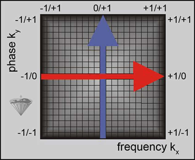
Figure 07-06:
The k-space raw data matrix consists of an area to be filled with the information nee­ded to form an MR image.

The coordinates of k-space are called spatial frequencies (measured in cycles per mil­li­me­ter). They are filled depending on gradient strength of the fre­quen­cy-en­­cod­ing gra­dient (readout gradient: red ar­row; x-direction) and phase-en­co­ding gra­dient (pre­pa­ra­tion gradient: blue arrow; y-direction), moving from low gradient strength (-1) to zero gradient strength in the center (0) and high gra­di­ent strength (+1).

In MR imaging, k is divided into three dimensions which define a do­main or a space: k_x, k_y, and k_z. Only k_x and k_y are commonly included.

The third, k_z, is the slice-selecting gradient which is mostly disregarded.

The points at the center of this raw data matrix represent small gradients; in­crea­sing the offset from the center corresponds to increasing gradient strength [⇒ Ljunggren 1983, ⇒ Twieg 1983]. Again, in an MR image the low spatial frequencies determine the gross signal levels (and hence contrast), while the higher spatial frequencies principally de­ter­mine the edge definition (sharpness), as shown in Figure 07-07. The definition of small objects is an integral part of the contrast and requires highspatial frequencies; thus, in this situation the high spatial frequencies also contribute to contrast.

The maximum signal intensity is recorded close to the center of k-space since the net read and phase gradients applied for these points are relatively small, resulting in less dephasing.

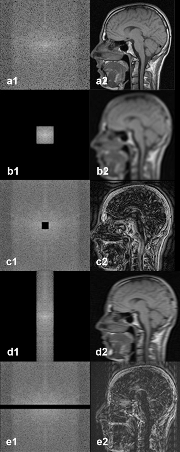
Figure 07-07:
k-Space with spatial frequency filtering.

a1|a2: Regular k-space with image re­con­struc­tion.
b1|b2: Same k-space as in (a) with filtering of the high frequencies; the reconstructed image has lost sharpness, it looks blurred, yet image contrast has hardly been affected.
c1|c2: Spatial frequency fil­te­ring of the low frequencies; the re­con­struc­ted image has lost image contrast, but image details have hardly been affected.
d1|d2: Low pass filtering in the readout direction, …
e1|e2: … high pass filtering in the preparation direction.

The signal amplitude (or mag­ni­tu­de) cor­res­ponds with the absolute brightness on the image because k-space is the re­pre­sen­ta­tion of the amplitudes of the sampled echoes. Therefore, the highest intensity is in the center.
Simulation software: MR Image Expert^®