


 onventional MR imaging is a slow imaging technique. Some people like it slow, others like it fast. Both styles have their advantages and disadvantages, as one sees in Figure 08-01. All of the classical imaging sequences have long scan times; for instance, the acquisition of a single spin-echo image takes between four and twenty minutes.
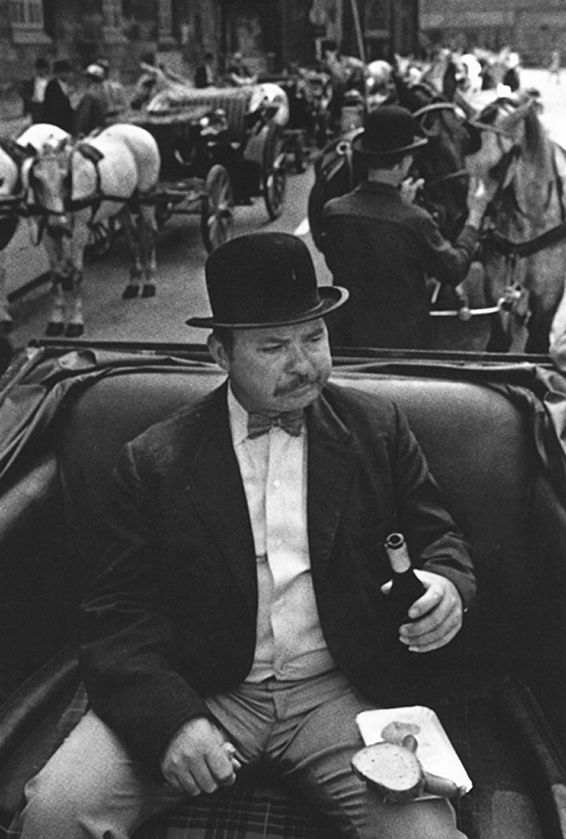
Figure 08-01:
This Viennese coachman prefers slower procedures; we would like to get it going a little bit faster. The question is: is the quality of the output better — or, in the long run, who gets better results?
 The principal constraints of imaging times are the long relaxation times on the one hand, and the desired signal-to-noise ratio and spatial resolution on the other hand. After 5×T1 of a tissue, the spins have nearly completely recovered. To get the optimum signal, one would have to wait for this period of time between each excitation pulse. Thus, to acquire images with a strong or even completely recovered T1 during TR requires relatively long TR values, particularly at high fields where T1 of tissues is longer than one second.
The equation on page 07-03 allows us to calculate the time needed to acquire the data for one image.
If TR = 2 s, NGy = 256, and NEX = 2, the data acquisition time adds up to 1024 seconds (i.e., 17 minutes and 4 seconds).
This used to be the common imaging time for a classical T2-weighted spin-echo image. As Figure 08-02 shows, many parameters influence imaging time and changing one of them will immediately have an interdependent effect on the others: Better spatial resolution with the same signal-to-noise, or better signal-to-noise with the same resolution, for instance, may require more averages and thus lead to a time penalty.
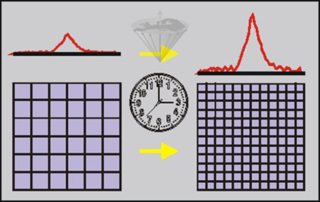
Figure 08-02:
Imaging time depends on a multitude of factors, among them signal-to-noise and spatial resolution.
From the early days of MR imaging, efforts were made to shorten the imaging time. Better signal-to-noise, for instance, was achieved by increasing the magnetic field strength of MR machines. Hardware, particularly coils, and software were also improved. Multi-echo multi-slice techniques were introduced to use the dead time during the long delays.
At the beginning of the 1980s, many physicists believed that rapid MR imaging would be impossible because of the limitations set by the relaxation times. Several seconds of recovery after every excitation was the main obstacle. Only in the mid-1980s did new ideas develop on how to accelerate imaging procedures.
To boost the understanding of rapid (or fast) sequences, let us recall some of the main factors of conventional MR imaging. Obtaining a signal which contains spatial information represents the first step in an MRI experiment. The next step is the manipulation of contrast in the images, which is achieved using a pulse sequence. Generally, the reconstruction technique and the pulse sequence are independent, so any pulse sequence can be combined with any reconstruction technique. For the purpose of understanding the basics of rapid imaging sequences, we will assume that the acquisition is performed with a 2D spin-warp sequence with selective excitation of one or more slices and the reconstruction with a 2DFT to produce a 2D image.
The form of the magnetic resonance signal is determined by a large number of factors, including proton density ρ, T1, T2, flow, and diffusion. By suitable preparation of the spins, we can emphasize the contribution of one or more of these factors.
The basic pulse sequences (spin-echo, inversion-recovery, partial-saturation) have to be modified for an imaging experiment since the FID signal has to be reformed in the presence of the imaging gradients by using either a spin- or gradient-echo sequence. This also provides sufficient time for the other position-encoding gradients (slice- and phase-encoding gradients in a 2D spin-warp experiment) to be applied.
The spin-echo sequence modified in this way produces a single spin-echo image, with the signal levels being mainly determined by the repetition time (TR) and the echo time (TE). By manipulating TR and TE, we can induce T1-weighted and T2-weighted contrast, respectively. This will be discussed in detail in the following chapters.
T1 contrast can also be generated by applying an inversion pulse (180°) and a delay (TI) prior to the excitation (90°) pulse. A 180° pulse always inverts the z-magnetization; in addition, when transverse magnetization is present, it also refocuses the transverse magnetization, leading to a spin echo.
To increase the amount of information available from a spin-echo sequence, we can apply a series of 180° pulses and create multiple echoes. Normally, each spin echo contributes one line of raw data in k-space to one image for each excitation. Thus for n spin echoes, n images are obtained. Multiple-echo sequences provide images with different contrast with increasing echo time. The various forms of the spin-echo sequence and their contrast behavior will be discussed in detail in the following chapters.


|

|
|---|