11-03 Diffusion Imaging

11-03-01 Background

Diffusion is but one mechanism of the transport phenomena on the molecular le­vel: fluid transfer, heat transfer, and mass transfer. It is very closely related to thermal conductivity and viscosity – and a vast and open scientific area [⇒ Bird]. The fundamentals of thermodynamics were explained by Fourier's law of heat conduction, those of viscosity by Newton's law of viscosity, and those of dif­fu­si­vi­ty by Fick's law of diffusion.

Fluids in the human body move in different ways, as bulk flow and perfusion in blood and lymph vessels, from the great vessels down to the capillary level, or as diffusion on the cellular level (Table 11-01). Tissue cells are surrounded by extracellular water through which small molecules shuttle between cells and the grand circulation. In the blood vessels the transport is active, mostly pumped by the heart, rather than passive, as in tissue, where it is controlled by diffusion in response to ever-changing chemical potentials.

Table 11-01:
Forms of fluid motion in the human body. Links marked in green.

Diffusion is defined as the process resulting from random motion of molecules by which there is a net flow of matter from a re­gion of high concentration to a region of low concentration (Figure 11-08). However, diffusion exists even in thermodynamic equilibrium.

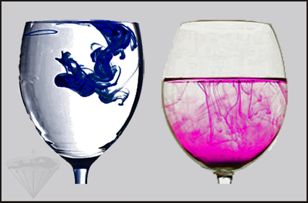
Figure 11-08: Distribution in water of blue ink from the top and potassium permanganete from the bottom of the glass. This kind of molecular movement is easily visible. Diffusion inside the body is far more difficult to explain, to conceptualize – and to unveil.

Displacement distribution is the fraction of particles that will move over a cer­tain distance during a given time. The rate of diffusion is governed by the dif­fu­si­vi­ty, D; its dimension is cm²/s. This coefficient depends on several factors such as size of particles and temperature; the most important factor is viscosity. Changes of intra- or extracellular viscosity induce alterations of diffusion, and thus can change image contrast in diffusion-weighted MR imaging (DWI).

 Diffusion had been a topic of research in NMR since the early 1950s.

Erwin L. Hahn showed that by forming a spin echo one could recreate the see­ming­ly irreversible NMR signal [⇒ Hahn]. He used three subsequent 90° pulses and tried to calculate T2 values with this method. However, these values were not reliable: they were distorted by molecular diffusion. Herman Carr found a way around this problem and to overcome diffusion with a train of 180° pulses after the first 90° pulse: The Carr-Purcell spin echo sequence [⇒ Carr], later mo­di­fied as the Carr-Purcell-Meiboom-Gill (CPMG) sequence by changing the pha­se of the 180° pulses relative to the initial 90° pulse [⇒ Meiboom] .

In 1968, Edward O. Stejskal and John Tanner proposed to apply pulsed gra­di­ents for easier and more precise measurement of spin echoes to study restricted diffusion. They called this method Pulsed Field Gradient, Spin-Echo NMR [⇒ Stej­skal].

The feasibility to visualize diffusion was discussed for a long time because it would allow differentiation between tissues according to their cellular structure. In 1986, Denis Le Bihan took this up and applied it to MR imaging [⇒ Le Bihan] by using appropriate gradient pulses to depict intravoxel incoherent motion (IVIM).

Diffusion is independent of the relaxation times and thus adds another factor to contrast.

11-03-02 Techniques

Tissue water diffuses randomly, but barriers such as cell membranes can in­flu­en­ce its diffusion and alter its random motion to a partly directed motion. For instance, diffusion in white matter shows a clear directional dependence be­cause, most likely, the myelin envelope covering the nerve fibers is virtually im­pe­ne­trab­le for diffusing water molecules. This leads to an anisotropically re­stric­ted motion [⇒ Moseley].

In more or less free diffusion, the displacment distribution is a bell-shaped (Gaussian) function; the more complex manner of diffusion in tissue cells is non-Gaussian. Diffusion-weighted imaging (DWI) is the elementary imaging me­thod; the next step is a pictorial depiction of the calculated Apparent Dif­fu­sion Coefficient, ADC. More complex methods include Diffusion Tensor Imaging (DTI) and related techniques such as Diffusion Tensor Tractography (DTT).

Diffusion-Weighted Imaging. DWI is commonly performed in the three or­tho­go­nal directions x, y, and z created by the existing gradient coils of the MRI ma­chine. A Carr-Purcell spin echo sequence is adapted to diffusion imaging by the ad­di­tion of two gradient pulses at a duration δ and a time difference Δ, the dif­fu­sion time (Figure 11-09).

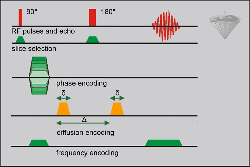
Figure 11-09:
Complete 2DFT spin-echo imaging experiment with pulsed diffusion encoding. δ is the duration of the diffusion-encoding gradient, Δ is the diffusion time interval (be aware that δ and Δ have dif­fe­rent meanings in other applications of MR imaging).

A phase shift dependent on the strength of the gradient pulse is induced by the first of the diffusion pulses. The second diffusion pulse is applied after the 180° pulse of the CP sequence (this 180° pulse reverses the phase change that was in­du­ced by the earlier pulse; cf. the explanation of the spin-echo creation in Chap­ter 6). After the first diffusion pulse, all proton spins in the excited area are de­pha­sed; now, diffusing spins move away randomly and, partly, out of the area of interest. Thus, they are not rephased by the second diffusion pulse, resulting in a decrease (attenuation) of the signal.

The b value is a term describing the diffusion sensitivity or the degree of the diffusion weighting of the final image: b ~ q²×Δ (dimension: s/mm²). The b va­lue is estimated on the basis of q, a vector in the direction of the diffusion. The length of this vector is proportional to the gradient strength.

Figure 11-10 gives an example of how diffusion influences contrast and its de­pen­den­ce upon gradient direction.

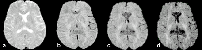
Figure 11-10: Transverse, increasingly diffusion-weighted images. (a) b = 0 s/mm² (no diffusion weighting); (b) b = 600 s/mm²; (c) b = 900 s/mm²; (d) b = 1200 s/mm².

On the images of Figure 11-10, regions with a high diffusion gradient show low signal intensity, regions with low or obstructed diffusion are brighter. This is the reason for contrast enhancement in diffusion weighted imaging (DWI), allowing for instance the early depiction of brain infarction. Appreciation of the contrast enhancement always requires the comparison of at least two images with dif­fe­rent b-values.

Pathologically increased diffusion patterns in the brain have been observed in infarction, tumors, edema, multiple sclerosis, and cysts. Diffusion changes in­di­ca­te ischemia at a very early stage. This finding is helping MR imaging become the modality of choice in patients with suspected brain infarction [⇒ Buxton, ⇒ Doran].

Apparent Diffusion Coefficient Imaging. The imaging method based on the apparent diffusion coefficient ADC serves as graphical illustration of the ability of protons to diffuse through tissue where they are restricted in their movement by, e.g., cell membranes or increased cellularity – which might be the case in tu­mors. ADC imaging requires at least two data acquisitions; its contrast behavior is reversed: areas of restricted diffusion are dark, those of free diffusion bright (Figure 11-11).

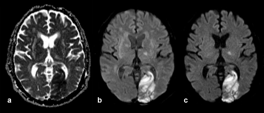
Figure 11-11:
Elderly patient with old and recent brain infarctions. New large infarction in left occipital lobe, also affecting other parts of the brain. (a) ADC image, the area of the infarction is dark; (b) diffusion-weighted image, b = 500 s/mm²; (c) diffusion-weighted image, b = 1000 s/mm². The area of the infarction is bright.

Diffusion Tensor Imaging. This method, also known as DTI or tractography is a mathematical processing technique of diffusion-weighted measurements. It is potentially valuable for brain diagnostics in areas of anisotropic diffusion, al­lo­wing the depiction of the direction and, possibly, interruption of tissue tracts. It is mainly applied to white matter axonal fiber bundles and, at the time being, re­mains a research technique [review articles: ⇒ Hagmann, ⇒ Nucifora]. DTI relies on algorithms that assemble two- or three-dimensional visualizations of main white matter axonal fiber bundles. It allows to delineate fiber bundles from each other, as well as from gray matter and CSF (Figure 11-12). For MR tractography fiber bundles must be aligned in one direction only and must not intersect. The tracts (fiber bundles) depicted on such an image are not the fibers per se, but local dif­fu­sion maxima.

Figure 11-12: Tractography calculated from DW imaging data. The signal of the neural tract is stron­gest when the diffusion gradient is di­rec­ted orthogonally to white matter bund­les, such as in the corpus callosum. The different diffusion directions (gradient directions) x, y, and z are color-coded in these images: x = red, y = blue, and z = green. It remains to be seen whether such ima­ges will have true clinical relevance.

There are a number of even more complex methods related to MR trac­to­gra­phy, such as diffusion spectrum imaging, q-ball imaging, and angular re­so­lu­tion imaging which are beyond this introduction to MR imaging.

Critical remarks. Pitfalls and problems of DTI are manifold and stretch from imperfect algorithms to motion artifacts. Crossing, converging or diverging white matter tracts might not be adequately depicted. In particular the hypothetical, complex algorithm-based variants of DWI should applied with caution. In re­search, DTI is an excellent complementary examination to functional brain ima­ging (BOLD imaging). The technique should only be used by qualified and cri­ti­cal scientific specialists.