


 he main objective of medical image processing is to facilitate the gathering or provision of information not easily seen, or not seen at all, on unprocessed images. Improvement of diagnostic performance to reduce the ever existing level of uncertainty is one of the main propelling forces in diagnostic imaging research.
Since the human visual-perception system is unable to perform multichannel analysis in order to achieve a new dimension, image processing developed in parallel to the introduction of MR imaging as a clinical tool.
Researchers wanted to detect any message, possibly hidden, in a single MR image or a series of MR images. Given that only minimal information existed about how to approach this scientific problem, the course of research was mostly empiric.
Historically, the following main lines of approach were followed:
 subtraction or superposition (overlay, data fusion) of multichannel images;
quantification of MR parameters, i.e., T1, T2 and proton density;
image segmentation and multispectral analysis;
3D visualization.
In general, the processing of digitally acquired images is aimed at improving pictorial information for human interpretation and (or) processing data for autonomous machine perception. Both aims have been targeted in magnetic resonance imaging and in both areas successful applications have been found.
All computed image-processing requires digitized imaging. In digitized radiology, the equivalent of a regular x-ray is taken and digitized directly by a specialized x-ray system. In nuclear medicine, CT, and MR, imaging slices through the human body are acquired and subdivided into volume elements. Then, the numerical signal from each voxel, in turn, can be translated into a distinct shade of the gray scale and be represented as a picture element in the final image (Figure 15-04). Both, single images or a series of similar images can be manipulated, e.g., by noise reduction, edge or contrast enhancement [⇒ Godtliebsen 1989].
In multichannel imaging, several channels representing n different parameters can be acquired simultaneously or by consecutive procedures, leading eventually to n images of exactly the same object (Figure 15-05).
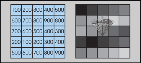
Figure 15-04:
Numerical image date output (left) turned into gray-scale image (right). Typically, one finds medical images with an image matrix of 256×256, 512×512, or 1024×1024 and 256 gray levels.
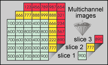
Figure 15-05:
If multichannel images of the same object are properly aligned, it is easy to compare or compute their signal intensities.
Image-processing allows the connection of picture element data of the same location in different images with changed parameters; known connections can be computed, e.g., by using appropriate equations.
Such procedures may extract additional information or allow quantification of data and thus a — perhaps — 'objective' definition of structures, tissues, or metabolic processes. Several single images can, e.g., be added to a new multispectral image (synthetic image) which does not necessarily add useful information or even depict reality (Figure 15-06).
Details on image processing can be found in a number of monographs [⇒ Gonzalez 2008, ⇒ Russ 2017].
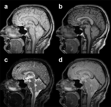
Figure 15-06:
Examples of multichannel images: (a) proton-density-weighted, (b) T1-weighted, and (c) T2-weighted images of a slice through the brain. The anatomic location of the pixels is exactly the same; according to image weighting the pixel representation is different.
(d) is a pixel-by-pixel compilation of images a-c. This synthetic image does not reveal any additional diagnostic information.
 There are different ways of classifying image-processing techniques, for instance, they can be defined by what they are supposed to achieve.
Types of techniques include noise reduction, image segmentation, feature extraction, and classification.
Whereas noise reduction is of vital importance for more noisy modalities like ultrasound, MR imaging has, due to a rapid development of MR hardware and software, not the same need for such techniques, perhaps with the exception of dynamic imaging (see Chapter 16).
However, image segmentation and image classification have found much more widespread use in MR imaging, partly due to the possibility of acquiring multichannel data suitable for such processing.
Another important group of image-processing techniques is image registration or image alignment, which sometimes employs image segmentation techniques to align images. Image registration is important for aligning multimodality data (for instance, nuclear medicine data and MR imaging data from the same patient) or registration of time series. A specific type of time series (dynamic contrast-enhanced MR imaging) is described in Chapter 16. Furthermore, time series can also be used for monitoring tumor growth or growth of bones in children.
Another important type of MR imaging time series is BOLD functional MR imaging (fMRI) of the brain. Image registration is routinely performed on fMRI data.


|

|
|---|