


 otion artifacts are the most frequently observed artifacts in MR imaging and have severely hampered the use of MR imaging for abdominal studies. They require ECG triggering being used for thoracic studies (Figure 17-07).
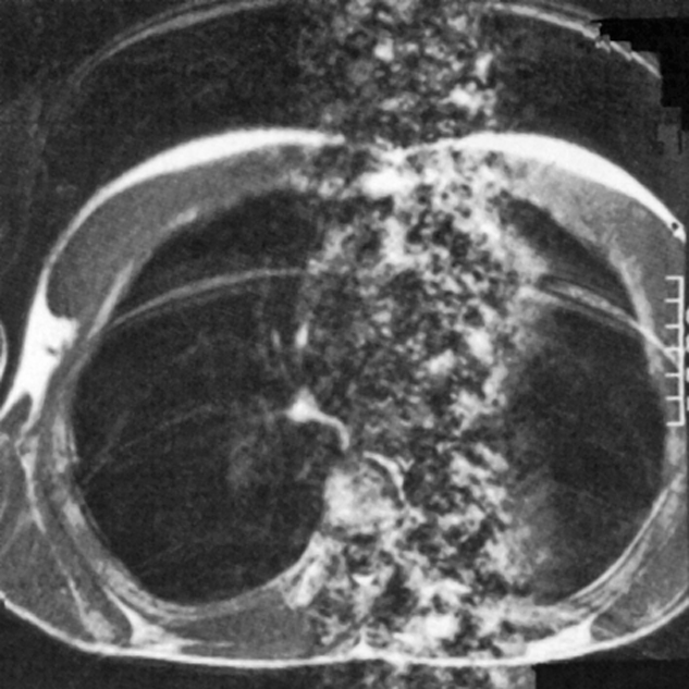
Figure 17-07:
Ghost images resulting from respiratory and cardiac motion with both sets of artifacts being oriented along the phase encoding gradient. The respiratory motion produces a number of distinct ghost images of the chest wall, while the cardiac motion results in the column of noise associated with the heart.
Motion can lead to blurring and ghost artifacts. Blurring of anatomical structures and interfaces is caused by averaging of moving structures (pseudo double exposure). This may obscure small lesions. Ghost images are partial copies of the parent image appearing at a different location; they are mostly caused by pulsatile flow.
Motion can be divided into two basic categories:
 motion occurring between acquisition of different lines in the study;
motion occurring between excitation and data acquisition.
The first category can be totally eliminated by physiological gating so that the data acquisition and motion are synchronous. This is widely used in cardiac studies and allows the generation of excellent, reproducible images of the heart cycle.
Respiratory gating has also been tried, but the much lower frequency of the respiratory cycle results in very long scan times. A number of other techniques monitor the respiratory cycle and select the phase-encoding steps in an order that minimizes the resulting artifact. The ROPE (Respiratory Ordered Phase Encoding) technique removes the periodicity of breathing upon k-space [⇒ Bailes 1985].
A technique developed later follows the normal sequence with a second acquisition which has no phase-encoding. This second echo, also called navigator echo, provides an indication of the amount of motion and can be used as the basis for a postprocessing procedure [⇒ Ehman 1989].
 All these techniques suffer from the fundamental shortcoming that they assume bulk motion, i.e., everything is moving in the same direction at the same speed, which is not true in the abdomen. Still, such techniques can improve image quality.
An alternative approach is to make the scan time short with respect to the respiratory cycle and hence limit the amount of motion. The ultimate example of this is echo-planar imaging where the image is formed from a single acquisition [⇒ Rzedzian 1986].
By using fast imaging techniques with acquisition times of a few seconds or less in conjunction with breath holding excellent images with few motion artifacts can be obtained.
Artifacts resulting from the second type of motion can be reduced by using motion-compensated gradients. The gradients in standard imaging sequences produce additional phase shifts for moving samples. Since the amount of motion will not be the same for each line of the scan (unless gating is used), a smearing of the signal in the phase-encoding direction will result.
By using a modified form for the read and slice gradients, one can remove this additional phase shift and as a result the artifact (MAST — Motion Artifact Suppression Technique) [⇒ Pattany 1987]. Its drawback is a slight prolongation of the minimum echo time.
The origin of flow artifacts is very similar to that of motion artifacts, namely that the blood and CSF flow can be pulsatile. Thus, different flow velocities will be present in different lines of the scan. The read and slice gradients induce a phase shift for flowing material, resulting in a range of phase shifts being produced in the course of a study [Van Dijk 1984]. The resulting artifact can take the form of a general smearing or a number of distinct artifacts in the phase-encoding direction (Figure 17-08).
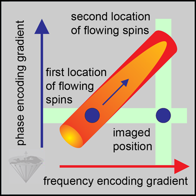
Figure 17-08:
The misregistration of flowing spins leads to the depicting of blood outside the vessel lumen: flow artifact.
The solutions are the same as for motion artifacts: the use of ECG gating to ensure that the same flow velocity is always observed and (or) the use of compensated gradients to null the phase shift from flowing material.
Flow artifacts are particularly severe in gradient-echo images since in a 2D study the flowing spins will not have experienced the preceding pulses and will therefore be fully recovered.
This leads to a very strong signal from the flowing (arterial) blood, and therefore to severe artifacts in the absence of gating and motion compensation (Figure 17-09). Venous flow also produces artifacts, but at a much lower level since this kind of flow is less pulsatile.
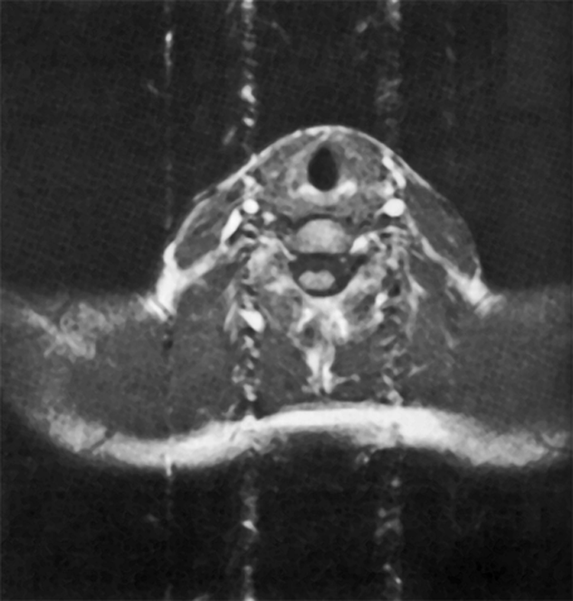
Figure 17-09:
Gradient-echo image of a neck with the phase encoding gradient oriented vertically. Flow artifacts are observed as a column associated with arterial vessels
Where flow of blood or CSF degrades the diagnostic quality of the MR image, artifacts should be eliminated. This can be achieved by presaturation.
Here, additional RF pulses are applied which saturate spins outside the imaged region. Thus, blood flowing into this region is saturated, which causes a reduction in blood signal intensity and in flow artifact. Usually this is performed on both sides of the imaged slice because blood can enter the slice from either direction.
Figure 17-10 depicts a theoretical example of parallel presaturation.
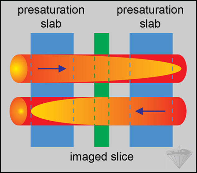
Figure 17-10:
Example of parallel presaturation. Presaturation pulses excite spins outside the slice to be imaged. Thus, flowing blood arrives already saturated when the spins in the slice of interest are exposed to the excitation pulse. The blood signal is suppressed and does not give rise to artifacts. The arrows indicate the direction of flow.


|

|
|---|