


![]() n MR spectroscopy experiments a sample is placed in a shimmed magnetic field to make it as uniform as possible. Now a particular molecule will give a signal of the same frequency at any point in the sample. Any frequency changes observed in the Fourier-transformed signal reflect chemical shifts within the sample which can be used to create analytical spectra.
n MR spectroscopy experiments a sample is placed in a shimmed magnetic field to make it as uniform as possible. Now a particular molecule will give a signal of the same frequency at any point in the sample. Any frequency changes observed in the Fourier-transformed signal reflect chemical shifts within the sample which can be used to create analytical spectra.
In imaging experiments we are not concerned with chemical shift information; chemical shift might even be counterproductive and considered artifact. To create an image from a patient, the magnetic resonance signal from the nuclei has to contain information about where the nuclei are positioned in the patient.
The MR equipment, as we have described it so far, does not provide us with any such information.
In Figure 06-03 we examine three small samples of water placed at different positions along the x-axis. Without the magnetic field gradient, applying an RF pulse produces a signal consisting of a single frequency; Fourier-transforming this signal gives a spectrum with a single peak.
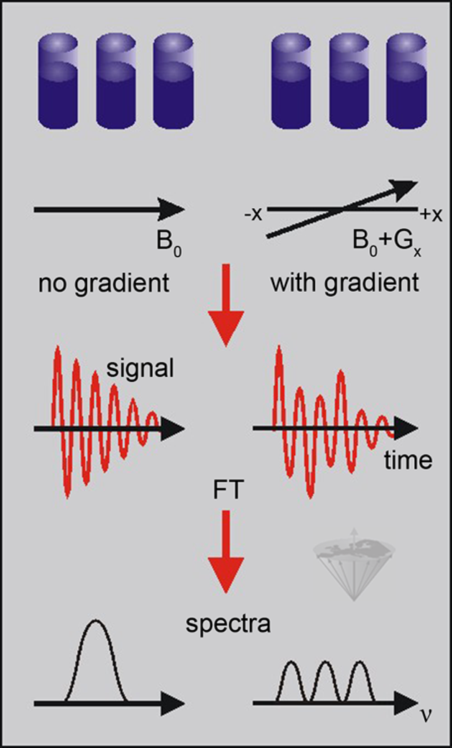
Figure 06-03:
The signals and spectra from three water samples at different positions along the x-axis with and without the application of a magnetic field gradient along the x-axis. In the presence of the gradient, the signals from the three samples are resolved, with the separation of the signals being dependent on their spatial separation in the x-direction and on the strength of the magnetic field gradient.
(FT = Fourier transform).
If a magnetic field gradient is imposed when we measure the signal, the signal consists of three different frequencies corresponding to the three different positions.
As stated before, the Larmor frequency is proportional to the magnetic field strength. If one varies the frequency of the signal by changing the magnetic field linearly across the sample, the frequencies at different locations will also vary linearly.
In our example, Fourier-transforming the signal gives a spectrum of three peaks corresponding to the three different sample positions. The frequency differences between the samples depend on their physical separation and the strength of the magnetic field gradient.
Today, all MR imaging methods utilize such magnetic field gradients for spatial encoding (Figure 06-04).
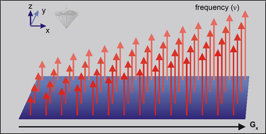
Figure 06-04:
Effect of field gradients: the frequency range is spread out.
In this case, the gradient follows the x-direction. The frequency in the center is the 'exact' resonance frequency.
The (magnetic) field gradients are generated by a set of coils positioned within the magnet. They can produce fields which vary uniformly along each of the three main axes (x, y, z).
At the center of the magnet, the resonance frequency is unchanged since the gradient has no effect at the center. On either side, the resonance frequency will be either higher or lower depending on the polarity of the gradient (Figure 06-05).

Figure 06-05:
Magnetic gradient fields are superimposed upon the static magnetic field. Different parts of the sample experience different magnetic field strengths. Only in the center of the sample is there no change of the static magnetic field, and thus of the resonance frequency ν₀.
These linear field gradients have a strength of up to 30 milli-Tesla per meter (mT/m) in standard 1.5 Tesla clinical systems, but much stronger gradients can be obtained by using smaller gradient coils, for specialized imaging methods, or at ultrahigh fields to avoid chemical shift artifacts.
Although the frequency variations produced by the gradients are very small compared to the resonance frequency, the range of resonance frequencies created is sufficient for high-resolution MR imaging. For example, to produce a frequency distribution of 25 kHz over a distance of 30 cm requires a gradient of only 2 mT/m.
The principle of the generation of a field gradient and the shape of gradient coils in a whole-body imaging system have been explained in Figure 01-04 and Figure 03-10.
Figure 06-06 shows how a pulsed magnetic field gradient is usually depicted in pulse sequence diagrams. In this case the gradient pulse is positive. Because there are three gradient directions x, y, and z, one can find gradients depicted in three 'electronic channels' in pulse sequence diagrams. Gradient pulses can consist of several different components.
The amplitude of the gradient is determined by the current flowing in the gradient coils. Shortening the rise time requires a faster rate of change of the voltage in the gradient coils.
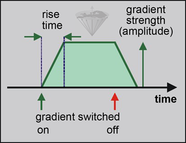
Figure 06-06:
Schematic representation of a pulsed field gradient used for pulse sequence diagrams.


|

|
|---|