


 igh-resolution magnetic resonance spectroscopists have measured T1 values since the middle of the last century. Such measurements can be performed in numerous different ways with various degrees of accuracy — in vitro (ex vivo) and in vivo.
In vitro measurements are done on a small samples, approximately 0.1-1.0 ml or slightly larger in volume, in an extremely homogeneous magnetic field.
A variety of methods has been developed to obtain maximal precision with minimal time consumption. Typically, 15 to 30 magnetization measurements are performed on the sample for different time delays, TI in inversion-recovery experiments or TR in partial saturation experiments. Based on these results, an observed T1 value is calculated, and the error limits are usually better than 5%.
T2 can be calculated with a single multiecho sequence. The more echoes one uses, the more accurate the measurement will be.
Calculations based on fast pulse sequences (so called black box sequences other than IR or SE) lead to rough estimates of T1, T2, T2* (and proton density) values. They might be reproducible when repeated, but the use of relaxation time values acquired with such pulse sequences is not advisable for scientific or clinical comparisons.
Magnet systems with larger bores allowed the examination of whole organisms, animals, and people, and a more physiological determination of relaxation time values than those of excised organs or tissues.
Relaxation time measurements were considered very important during the first years of commercial (medical) MR imaging. All machines were programmed to create true T1 and T2 images (i.e., T1- and T2 mapping), based on SE and IR sequences.
Very early, test objects and the protocols for their use to allow the measurement of T1 and T2 precisely and accurately were introduced in the framework of an extensive European project. The findings were sobering, but scientifically predictable [⇒ EEC 1988].
In particular, the accuracy and precision with which the relaxation times T1 and T2 could be measured from the images were found to be rather disappointing. Smaller comparison studies followed. It became clear that relaxation time values were not the claimed invaluable addition to diagnostics, and this 'standard' application was skipped [⇒ Lerski 1988].
A similar multi-center trial was repeated more than 30 years later. Phantom studies — newly introduced in the United States — described the same imprecision and irreproducibility of T1 measurements acquired on different MRI machines, most pronounced when rapid techniques for the estimation of relaxation constants were used [⇒ Keenan 2021] (cf. Rapid relaxation estimation techniques).
 Localization. One of the major problems of in vivo relaxation time measurements is the localization of the volume to be observed.
Actual accuracy of in vivo measurements depends on the number of points acquired and the quality of localization. Localization is relatively uncomplicated in little or non-moving organs such as the brain, but demanding and partly impossible (in particular at high/ultrahigh fields) in organs with complex movement patterns such as the heart.
Details of localization techniques are given in Chapter 6.
Relaxation Time Values and Proton Density Calculation. The current most dependable method used to obtain a T1 image (T1 map), i.e., an image whose picture elements represent pure T1 values, relies on a mathematical manipulation of separately obtained images with different T1 influence. Measurements are easier and more accurate at low and medium fields, because T1 values are shorter, ECG triggering less complicated, and artifacts less pronounced at these fields.
Typically, two to four images are used and the signals mathematically processed to calculate pure T1 values. Bearing in mind that in vivo relaxation can be multiexponential, it is somewhat inadequate to perform the analysis by such a limited fit to an exponential curve.
T2 images are calculated from the images of a multi-echo series, e.g. CPMG. In clinical settings, usually four or eight echoes are applied.
Diffusion, flow, and multiexponential decays are hardly ever taken into account in the fits and noise as well as motion artifacts add to inaccuracies.
Matrix size and slice thickness as well as partial volume effects are limiting factors in relaxation-time measurements in vivo. Variations within the same lesion related to vascularity, necrosis, and cell behavior (macroscopic compartmentalization) contribute to the overlapping of relaxation times values.
All methods relying on slices through the examined object will have as additional error source partial volume effects from the edges of the slices; the only method which avoids this slice problem is the true 3D volume imaging method.
Standard deviation in fitting, artifacts, and variations in the selection of volume elements by the operators are all possible sources of error (Figure 04-21).
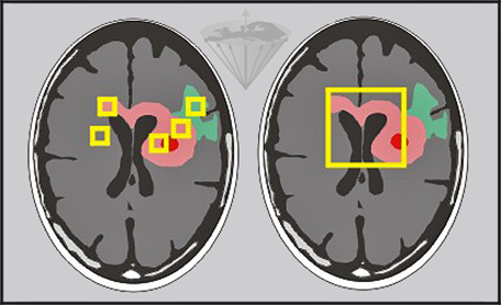
Figure 04-21:
Relaxation time measurements in vivo can be performed pixel by pixel and by regions of interest of different size.
Left: Small regions of interest covering edema (green), tumor (pink), necrosis (red) and other pathologies.
Right: Large region covering major parts of the tumor.
Furthermore, similar lesions may have more than a single exponential relaxation rate, e.g., brain tumors and multiple sclerosis plaques. This is not unexpected, considering the heterogeneous nature of tumors — and tissues in general.
Reproducibility of such measurements is also limited.
The multilayered complexity of factors and features influencing and creating relaxation time and proton distribution changes is not completely understood yet [⇒ Springer 2014]. A simplified view offered by Koenig suggests that water molecules can wander rather extensively by thermally-induced diffusion throughout the intra- and extracullular regions of tissue, and that the exploration is rather thorough in a time of the order of T1 (or even T2).
Another concept is the highly structured water, restrained for a significant time in a geometry defined by various ionic and molecular constituents of the cytoplasm [⇒ Koenig 1985, 1988].
However, some features of the T1-dispersion do not fit easily into these concepts, for instance cross relaxation phenomena that lead to quadrupolar dips in the T1-dispersion plot. They are dependent on field strength and temperature (Figure 04-22) [⇒ Rinck 1988]. More about the dependence of relaxation times on static field strength and its influence upon contrast can be found in Chapter 10.
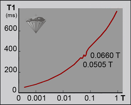
Figure 04-22:
The dispersion of T1 in tissues (ms) versus field strength (log Tesla) is not as monotonic and smooth as shown e.g. in Figure 04-04 and Figure 10-16.
This high resolution nuclear magnetic relaxation dispersion (NMRD) curve of a multiple sclerosis tissue sample reveals two dips (quadrupolar dips) at 0.0505 and 0.0660 T (2.1 and 2.8 MHz) where the otherwise steady increase of T1 is interrupted.
Relaxation time and proton density values can be used to create synthetic or simulated images for training and teaching purposes.
In clinical routine, people often talk about T1, T2 or proton-density images. The correct terms are T1-weighted (or dependent), T2-weighted (or dependent), and proton density (ρ)-weighted (or better, intermediately weighted) images, because these images have only a certain T1, T2, or proton-density dependence. They are not calculated pure relaxation time or proton density images. Chapter 10 will explain this in detail.
Figures 04-23c and d are T1-weighted and T2-weighted images, to be compared with the pure T1 and T2 images of Figure 04-23a and 04-23b.
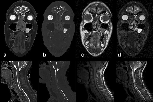
Figure 04-23:
(a) Calculated (pure) T1, and (b) calculated (pure) T2 image. Figures (c) and (d) show T1- and T2-weighted images.
Top row: Images of a patient with a polyp in the left paranasal sinus.
Bottom row: images of a cervical spine.
Pure T1 and T2 images are of very limited diagnostic value. Multiparameter weighted images are far more valuable for clinical diagnosis and commonly used in patient studies.
Simulation software: MR Image Expert®


|
Chapter 4 — Page 6 |

|
|---|