


 number of possible slice configurations in multiple slice imaging is depicted in Figure 06-18. Provided there is no overlap between the slices, then each slice should be totally independent of the other slices.
If there is an overlap, the RF pulses used for excitation of the different slices interfere with each other and interrupt, for instance, the T1 recovery in adjacent slices, leading to reduced signal-to-noise ratio and influencing signal intensities.
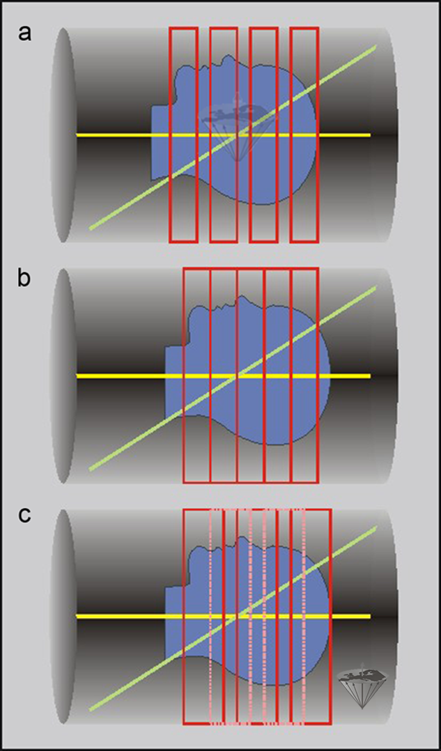
Figure 06-18:
Multiple slices: (a) multiple slices with wide gaps; (b) multiple contiguous slices; and (c) multiple overlapping slices.
Commonly, a small gap is retained between slices to avoid this kind of crosstalk, or the excitation pulses are distributed over two packages; the first one excites the odd, the second one the even slices.
In many pulse sequences, there is a quite long TR between each excitation of a particular slice while the magnetization recovers. Because of the relatively long T1 relaxation time of tissues, a delay of up to three seconds may be necessary before repeating the excitation. To make the most efficient use of this time, we can excite a number of parallel slices in each interval, which is achieved by changing the frequency of the RF pulse. This procedure can be repeated to produce a series of slices (Figure 06-19).
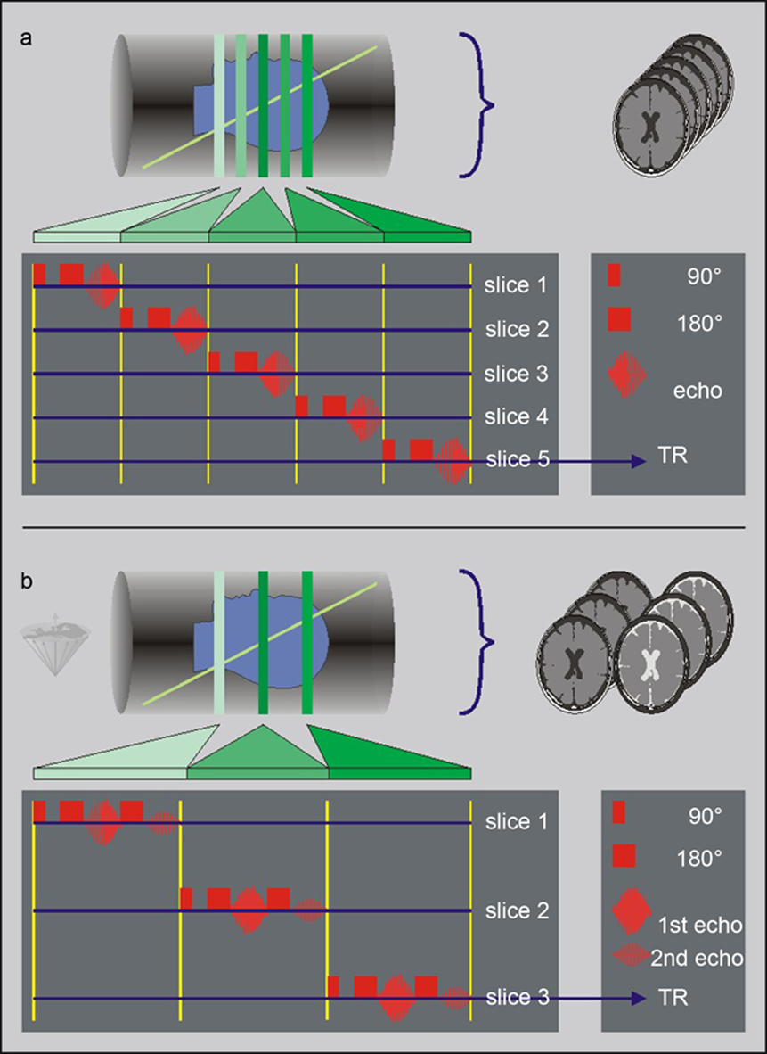
Figure 06-19:
Top: Excitation of multiple slices within one TR cycle (SE pulse sequence: multi-slice single echo). In this case, five slices can be excited within one repetition cycle. The excitation frequency of the individual pulses is slightly changed so that only selected nuclei, and thus slices, are excited (cf. Figure 06-17).
Bottom: Excitation of multiple slices within one TR cycle (SE pulse sequence). In each slice, one echo has been added to create a multi-slice double-echo sequence. The number of slices has been reduced to three because of the time restriction.
The number of slices obtainable can be calculated by dividing the repetition time TR by the time required for each slice. For example, if TR = 400 ms and TE = 50 ms, the theoretically possible number of slices is eight (in practice seven, since each slice requires slightly more than TE). If the repetition time is long enough, not only several slices but also several images with increasing echo times per slice can be created.
This is known as multi-slice multi-echo sequence.
Commonly in an investigation of the brain, 15 or 16 parallel slices in the transverse view with two echoes are acquired. The repetition time (TR) is between 2000 and 3000 ms, the times of the two echoes (TE) are 20 and 80 ms.
Multiple slice imaging is not restricted to spin-echo sequences, but can be performed with practically all pulse sequences.
One can add inversion pulses to create inversion-recovery images with a relatively long inversion time (TI); during this time, additional slices can be inverted. However, usually the number of slices is limited in IR sequences.


|

|
|---|