


 ith the implementation of gradients, we can locate the nuclei in our sample, but we also have added a problem. If we switch on a gradient after the RF pulse, the mere act of switching on the gradient significantly reduces the magnitude of the magnetic resonance signal from a sample (Figure 06-07).
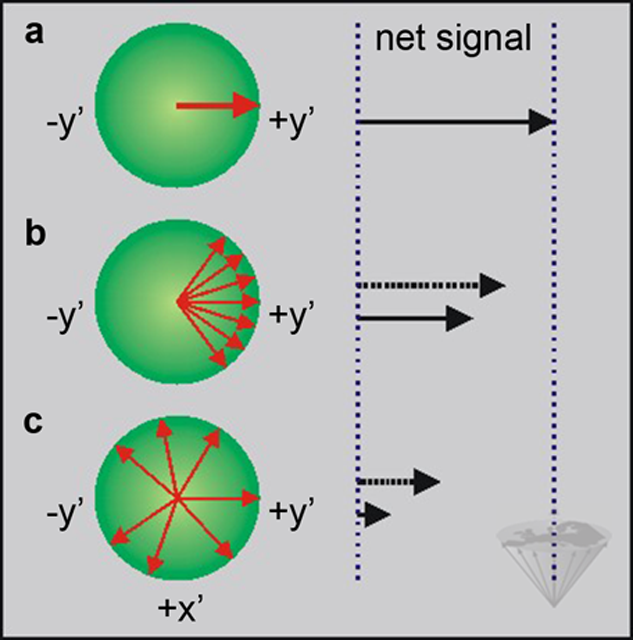
Figure 06-07:
Dephasing produced by the application of a gradient.
(a) The signal is initially aligned along the y'-axis and decays at a rate determined by T2.
(b) If we turn on a magnetic field gradient, we observe an accelerated spreading of the spins.
(c) Increasing the time delay increases the fanning out of the signal.
The solid arrows represent the net signal. The dotted lines in (b) and (c) are the signal that would be measured in the absence of the gradient.
Ideally, the signal will remain aligned along the y'-axis and decay at a rate determined by T2. However, even small imperfections in the magnetic field cause a spreading out (dephasing) of the magnetization.
The dephasing of the spins is amplified by the field gradients we want to use to localize the spins. Thus, by the time we have a stable gradient and can measure the signal in the presence of the gradient, we will have little or no net signal.
To avoid this problem, we have to reform the signal in the presence of the magnetic field gradient. This can be achieved using either a spin-echo or a gradient-echo pulse sequence, thus restoring the original signal in the presence of the gradient, allowing its detection and spatial encoding.
As we have already seen in Chapter 4, a spin echo is formed by applying a 180° pulse at a time τ after a 90° pulse. Following the 90° pulse, the magnetization vectors spread out because of the variations in resonance frequency caused by field inhomogeneities (ΔB₀).
Applying the 180° pulse reverses the dephasing, so that at a time τ after the 180° pulse, these effects are cancelled out and an echo is formed: only T2 decay reduces the intensity of the echo.
Complete rephasing only occurs at the center of the spin echo. With increasing distance from the center the effects of field inhomogeneities grow.
The spin-echo sequence also refocuses chemical-shift effects at the center of the spin echo.
Therefore, the water and fat signals will be in phase at the echo center. In a non-imaging spin-echo experiment, the dephasing effects in the two halves of the experiment before and after the 180° pulse are equal.
In an imaging experiment, we can control both the duration and the amplitude of the imaging field gradients and arrange for the gradient areas to be equal (Figure 06-08).
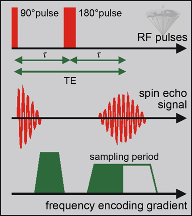
Figure 06-08:
Spin-echo experiment with balanced gradients during the sequence. The (green) gradient pulse between the 90° and 180° pulses equals the green area of the gradient after the 180° pulse. Since the 180° pulse induces a phase reversal, the effects of the two gradients cancel at the center of the spin echo. Therefore, a spin echo forms in the presence of a gradient.
We do not necessarily need a 180° pulse To create an echo. Another possibility is using field gradients. This leads to gradient echoes, which are widely used in so-called rapid (or fast) imaging sequences.
Following an RF pulse, the signal decays due to the combined action of T2 decay and local field inhomogeneities. This effect is described by T2*. By altering the polarity of the gradient, we change the direction of the induced precession, the spins start rephasing, and at the echo time TE grow into a gradient echo (Figures 06-09, 06-10, and 06-11). To create such an echo, the areas of the gradients with different polarities must be equal [⇒ Hutchison 1980].
A gradient-echo (GRE) experiment measures a delayed reformed version of the FID. This is necessary due to the gradient switching. Unlike spin echoes, with gradient echoes the effects of field inhomogeneities are not cancelled out. The signal decays faster; therefore, GRE experiments require a relatively short echo time.
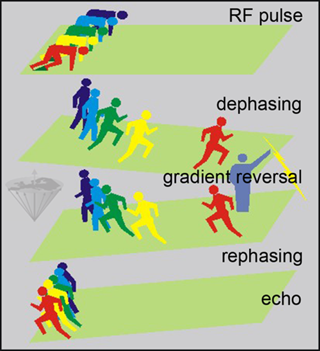
Figure 06-09:
Formation of a gradient echo using the example of the runners we have already used to demonstrate the creation of a spin echo (cf. Figure 04-18).
All participants start together; they begin to separate from each other, accelerated by the gradient. By the reversal of the gradient, they are recalled: they turn around at their present position and run back to the starting line.
Unlike in the spin-echo experiment, they return on their own track to form a gradient echo.
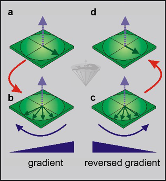
Figure 06-10:
Formation of a gradient echo in the absence of local field inhomogeneities. The presentation is counter clockwise !
(a) Immediately after the RF pulse the transverse magnetization is strong; the spins are in phase.
(b) The spins begin to dephase; the application of a field gradient accelerates this process. The net magnetization vanishes.
(c) The gradient is switched to the opposite polarization and the spins begin to rephase, until
(d) a gradient echo is formed.
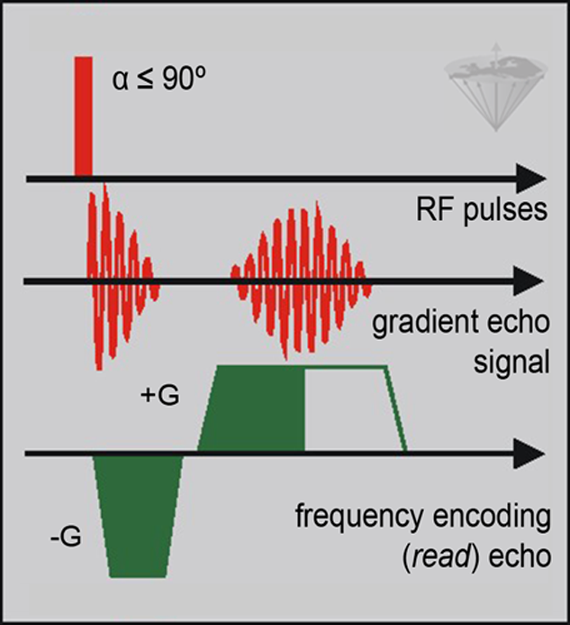
Figure 06-11:
Formation of a gradient echo.
Instead of the 180° pulse, a gradient pulse (-G) is used followed by a second gradient pulse of opposite polarity (+G).
For spin echoes, the signal decay is determined by T2, since the effects of local field inhomogeneities are cancelled out. With gradient echoes the signal decay is determined by T2*; it is always less than T2. More about T2* can be found in Chapter 4 at Table 04-01 and T2*.


|

|
|---|