


 or many clinical indications, rapid imaging sequences are essential to avoid long imaging times, which can cause motion artifacts, be inconvenient to patients — and reduce patient throughput. Imaging time can drop from several minutes per standard SE image to seconds or even milliseconds. The number of specific indications of particular rapid pulse sequences has steadily increased over the last few years.
GRE sequences were the favorite rapid imaging sequences; however, the popularity of sequences in the RSE and EPI families is constantly increasing.
For faster imaging, the number of averages, the number of matrix points or image lines, or the repetition times have to be shortened. In general, signal-to-noise ratio and spatial resolution will worsen with faster imaging methods, but as stated, a good clinical diagnosis does not necessarily require beautiful image quality, but sufficient image quality. The main contrast parameters of conventional and rapid sequences are summarized in Table 10-05. Actual weighting of the sequences depends on a number of factors and might not be available on all MR imaging machines.
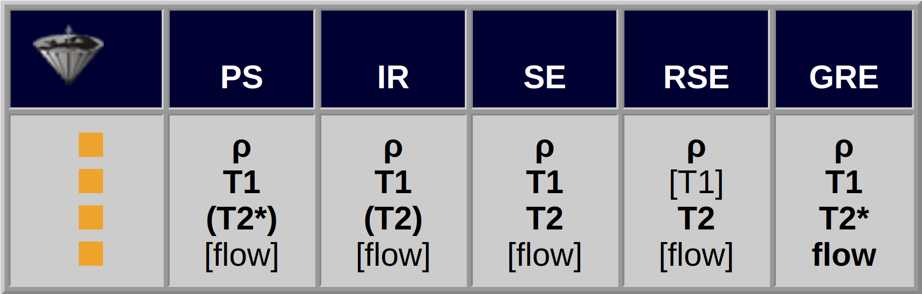
Table 10-05:
Pulse sequences and their contrast dependence. The signal of all pulse sequences is influenced by ρ and by bulk flow.
The T2*-dependent PS sequence equals a GRE sequence.
GRE sequences take advantage of the saturation of the spin system when TR is shortened. The signal intensity after a series of 90º pulses becomes weaker, until an equilibrium (i.e., the saturation) is reached. Under these conditions, pulse angles smaller than 90° are more effective.
It was unexpected that shortening TR below 100 ms, even below 10 ms, still provided images with a signal-to- noise ratio which was sufficient and allowed diagnostic assessment.
Gradient-echo sequences of this kind, with such short TR, have been dubbed FLASH sequences [⇒ Haase 1986]. They are commercially available under several different trade names (see Table 10-06 and List of Abbreviations).
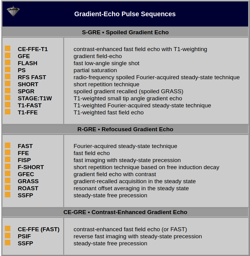
Table 10-06:
Some rapid imaging techniques correlated to the respective generic pulse sequence. Note: In this context, contrast-enhanced refers to the RF pulse sequence; is does not mean enhancement with a contrast agent. A detailed review can be found in a paper by Chavhan and collaborators [⇒ Chavhan 2008].
Signal intensity in rapid imaging sequences can be calculated with the following equation, if TR is shorter than T1 but longer than T2* or when gradient/RF spoiling is applied to remove transverse coherences:
where α is the flip angle, TR the repetition time, T1 the longitudinal and T2 the transversal relaxation time.
FLASH sequences add a fourth parameter to TR, TE, and TI: the pulse or flip angle α, also called FA.
Similar to SE sequences, GRE sequences can be weighted depending on repetition and echo times, the exact pulse sequence and the pulse angle. However, there is one big difference: whereas SE and RSE sequences reflect true T2 in their T2-weighted images, GRE sequences show only T2* contrast.
Figures 10-12 and 10-13 depict the typical signal intensity behavior of a GRE sequence, in this case a spoiled FLASH sequence. Commonly, the signal intensities reach a maximum between 30° and 60°.
As we have seen with the signal intensity and contrast behavior of SE sequences, best contrast is not necessarily obtained at the point of highest signal intensity. This is also the case in GRE sequences, as the contrast behavior of the brain images of Figure 10-13 shows. At the greatest signal intensity, there is poor or no contrast.
It turns out that images acquired using the Ernst angle tend to have rather poor contrast. Higher flip angles have to be used to improve the contrast. The effect of this is a reduction of the signal left along the z-axis after the RF pulse. Thus, the signal level depends on the rate at which the signal recovered during TR; it is strongly T1-dependent. The image series in Figures 10-12 and 10-13 give an overview of how contrast changes with increasing flip angle.
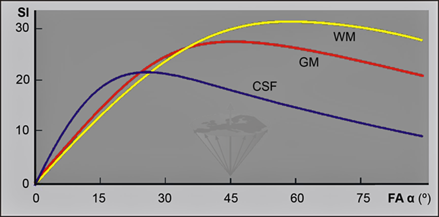
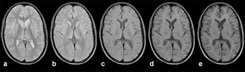
Figure 10-12:
Gradient echo sequence (spoiled GRE). TR = 400 ms; TE = 20 ms. B₀ = 1.5 T. Because of the three variables available, there are nearly unlimited possibilities for changing image contrast. Generally, at low flip angles proton density dominates contrast, at high flip angles T1 becomes more important.
Images (through the brain of a normal volunteer): (a) α = 15°; (b) α = 30°; (c) α = 45°; (d) α = 60°; (e) α = 75°
Simulation software: MR Image Expert®

Figure 10-12-Video:
Animation: Eleven images; α between 8° and 88°. Note that these are simulated images: Both on the picture sequence of Figure 10-12 and on the animated sequence image noise has been removed.
Simulation software: MR Image Expert®
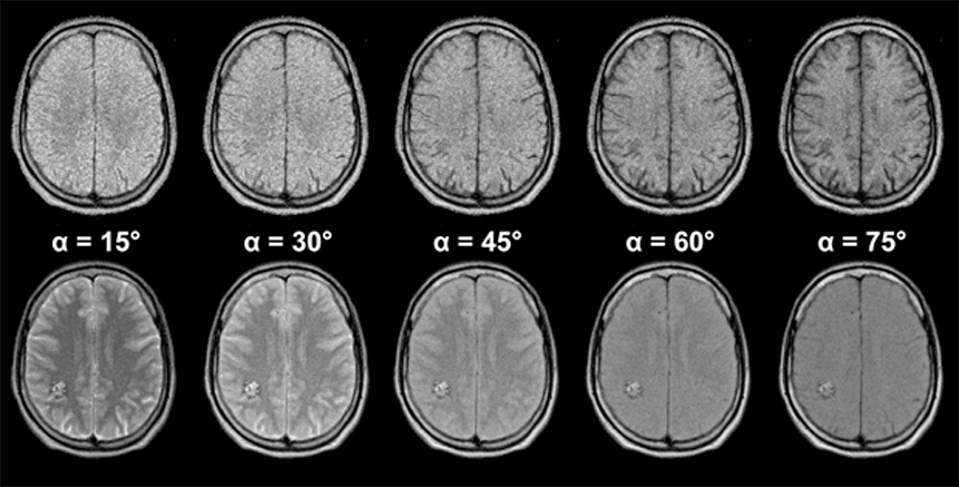
Figure 10-13:
Gradient echo pulse sequence (spoiled GRE) through the brain of a patient with a vascular malformation in the right occipital hemisphere.
The upper image series was taken with an echo time TE = 20 ms, the lower series with an echo time TE = 120 ms (B₀ = 1.5 T). The lesion is nearly invisible in the image series with short TE, but well delineated in the series with long TE.
The choice of the appropriate pulse sequence parameters is pivotal in MR imaging. Many different sequences can be applied for different diagnostic questions. In many instances, their contrast behavior has been recorded empirically and the sequence and specific sequence parameters have been included in special clinical imaging protocols.
Simulation software: MR Image Expert®
GRE sequences can provide sharp contrast between the CSF compartment of the spine, the spinal cord, and the peripheral spinal column. The myelogram effect of the T2*-weighted images allows a fast screening for disk protrusions and is one example of clinical applications of GRE.
SE and, in some instances, RSE sequences commonly yield sharper spatial detail, and contrast of GRE sequences generally is inferior to that of SE sequences.
T1 contrast can be enhanced by contrast agents.
The creation of T2*-weighted contrast is hampered by field inhomogeneities, which are not refocused by the gradient echo. The inhomogeneities solicit short echo times and limit the use of long echo times necessary for T2*-weighting. Reduction of TR shorter than T2 leads to the generation of transverse coherences which can either be spoiled or refocused, as described in Chapter 8.
Spoiled FLASH sequences (cf. Table 10-06) remove the effect of the transverse coherences, usually by the application of spoiler gradients, to give genuine partial saturation contrast. Refocusing GRE sequences incorporate the transverse coherences into the observed signal, and thus have a better signal-to-noise ratio. However, the basic refocused FLASH sequence generally has rather poor contrast (which depends on T1/T2). The contrast-enhanced version, CE-FLASH, offers additional T2 contrast, the amount of T2-weighting being determined by TR and T2. The T2-weighting is greatest at longer T2 values (e.g., 30-60 ms), but the signal-to-noise ratio is poorer than at short TR values.
GRE sequences are exquisitely sensitive to magnetic susceptibility (e.g., depicting hemorrhage and blood degradation products) and to flow phenomena (angiography).
As we have seen in the SE sequences, one can hide and miss pathological changes by choosing the wrong pulse sequence. This also holds for rapid sequences. If we select a T1-weighted sequence, we cannot distinguish a lesion which possesses a similar T1 to its neighboring tissues. If we apply a T2*-weighted sequence, we cannot delineate a lesion with a T2 close to the T2 of its surroundings. The signal intensity of the vascular malformation in Figure 10-13 is a good example of this problem.
Table 10-07 summarizes the features of a standard GRE (FLASH) sequence at high field (1.5 Tesla). A fine review of fast and ultrafast gradient echo sequences (including additional sequences to those mentioned here) was published by Nitz [⇒ Nitz 2002].
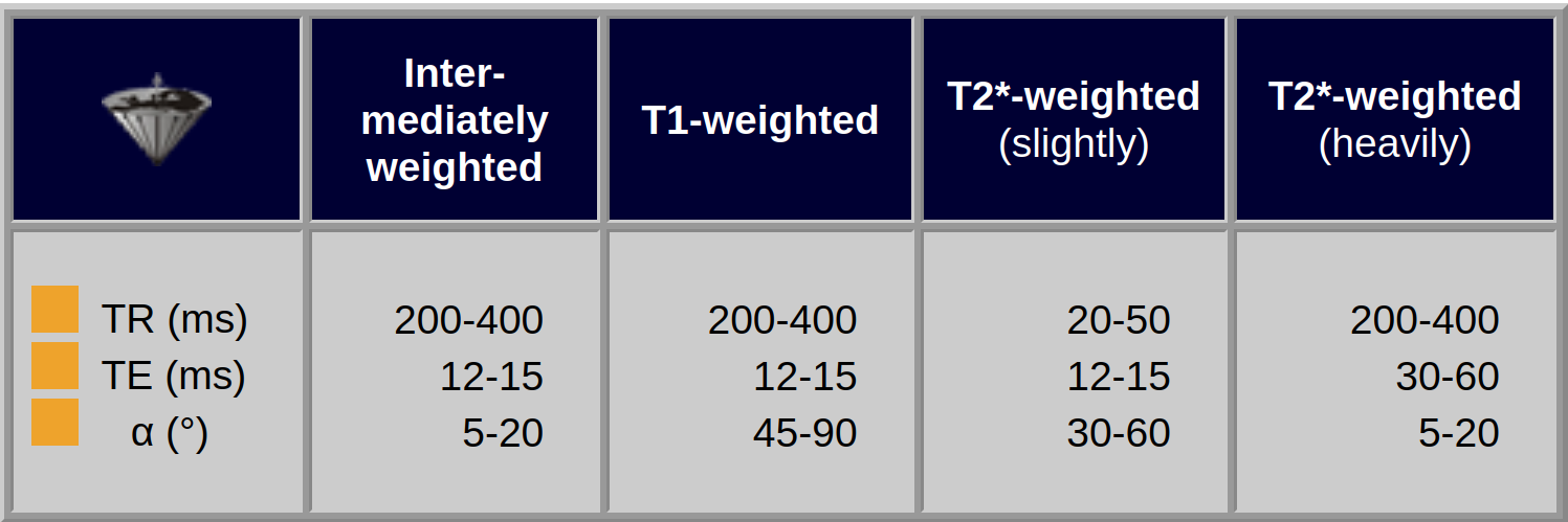
Table 10-07:
Approximate contrast characteristics in a standard GRE sequence at high field (1.5 Tesla).
In snapshot gradient-echo scans, the signal evolves to different levels during the scan. Therefore, by manipulating the starting value one can alter the form of the evolution and thus the image contrast. The most commonly used preparation pulse is a 180° inversion pulse.
3D MP-RAGE (three-dimensional magnetization-prepared rapid gradient echo) was introduced by Mugler and Brookeman in 1990 [⇒ Mugler 1990]. The MP-RAGE sequence combines a 3D-inversion recovery pulse and N equally-spaced readout RF pulses of a specific flip angle with an echo spacing τ. The pulse cycle within the repetition time, TR, consists of the following components:
where τ is echo spacing time, N the total number of readout RF pulses, TI the time interval between the inversion recovery pulse and the first RF readout pulse, and TD an adjustable delay time.
Image contrast is a function of N, TI, τ, the flip angle and the temporal position of the readout RF pulse, as well as the regular factors influencing contrast such as relaxation times. Generally, the total number of RF pulses N is related to the spatial resolution along the slice direction.
In commercial machines, the k-space strategy, including k-space trajectory and sampling order, is constrained to a few choices ('black box' equipment). Often the theoretically achievable best signal cannot be obtained on such machines.
In the MP-RAGE sequence, the effective inversion recovery time (TIeff) is a major determining factor of image contrast. It is defined as the time interval between the inversion recovery pulse and the RF read-out pulse for k-space center (Figure 10-14).
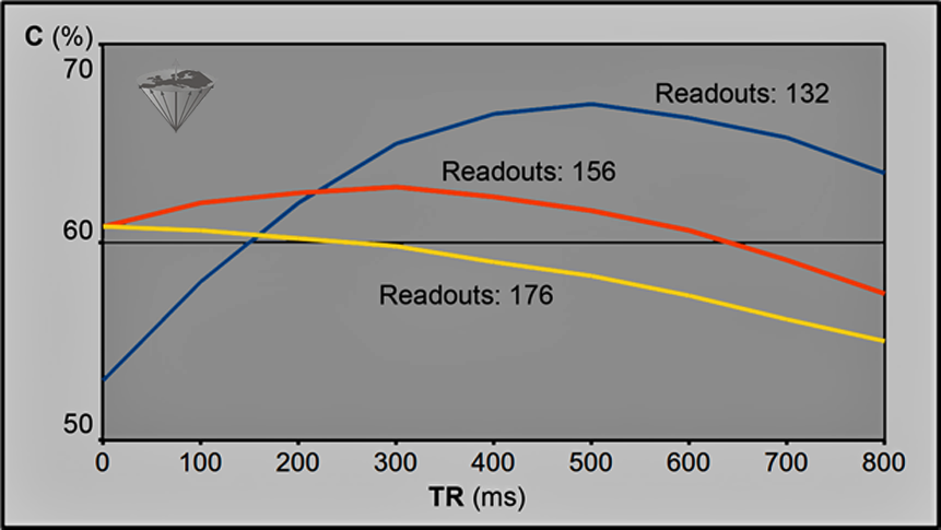
Figure 10-14:
3D-MP-RAGE. Simulated contrast between gray and white matter at 3.0 Tesla as function of TI for a total number of readout RF pulses of 176, 156, and 132, respectively. The interval time between readout RF pulses was set to 10 ms; the flip angle to 12°. To get decent T1-weighted contrast, the flip angle should be kept lower than 20° in this kind of pulse sequence. Contrast between tissues changes drastically with changes of TI as well as other parameters, e.g., T1 relaxation and field strength.
A good overview of the contrast behavior as well as of the basics of this pulse sequence was given by [⇒ Wang 2014].
Other Rapid Imaging Sequences. Chapter 8 describes a number of other fast imaging sequences, such as EPI.


|

|
|---|